机器学习题解（一）—— 线性回归与逻辑回归

ex1.m

Part 1: Basic Function

Modify warmUpExercise.m to return a 5 x 5 identity matrix

1	A = eye(5);

Part 2: Plotting

Plot the training data into a figure in plotData.m

data = load('ex1data1.txt')
x = data(:, 1);y = data(:,2)
m = length(y)

plot(x, y, 'rx', 'MarkerSize', 10);
ylabel('Profit in $10,000s')
xlabel('Population of City in 10,000s')

Part 3: Cost and Gradient descent

complete the code in the file computeCost.m, which is a function that computes J(θ)

1	J = sum(((X * theta) - y).^2) / (2 * m);

Perform a single gradient step on the parameter vector theta in gradientDescent.m

1 2	for iter = 1:num_iters theta = theta - alpha * (1 / m) * (X'* ((X * theta) - y) );

ex2.m

Part 1: Plotting

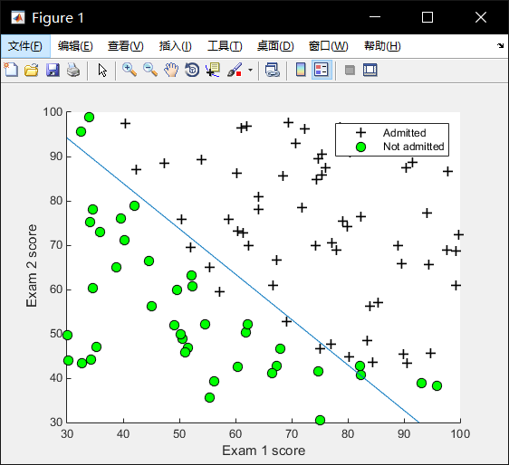
Plot the positive and negative examples on a 2D plot, using the option ‘k+’ for the positive examples and ‘ko’ for the negative examples

1
2
3

positive = find(y == 1); negative = find(y == 0);
plot(X(positive, 1), X(positive, 2), 'k+','LineWidth', 1.2, 'MarkerSize', 8);
plot(X(negative, 1), X(negative, 2), 'ko','MarkerFaceColor', 'g', 'MarkerSize', 8);

Part 2: Compute Cost and Gradient

Compute the sigmoid of each value of z (z can be a matrix, vector or scalar)

1 2	% Y = exp(X) 为数组 X 中的每个元素返回指数 e^x g = 1 ./ (1 + exp(1) .^ (-z));

Compute the cost of a particular choice of theta. You should set J to the cost

1
2
3

J = (1 / m) * sum(
	-y .* log(sigmoid(X * theta)) - (1 - y) .* log(1 - sigmoid(X * theta
)));

Compute the partial derivatives and set grad to the partial derivatives of the cost w.r.t. each parameter in theta

1 2	for j = 1:size(theta) grad(j) = (1 / m) * sum((sigmoid(X * theta) - y) .* X(:, j));

Part 3: Optimizing using fminunc

Part 4: Predict and Accuracies

Complete the following code to make predictions using your learned logistic regression parameters. You should set p to a vector of 0’s and 1’s

1	p = sigmoid(X * theta) >= 0.5;

ex2_reg.m

Part 1: Regularized Logistic Regression

Compute the cost of a particular choice of theta. You should set J to the cost
- tip: In Octave/MATLAB, recall that indexing starts from 1, hence, you should not be regularizing the theta(1) parameter (which corresponds to θ0) in the code

1	J = (1 / m) * sum(-y .* log(sigmoid(X * theta)) - (1 - y) .* log(1 - sigmoid(X * theta))) + (lambda / (2 * m)) * sum(theta(2:size(theta)) .^2);

Compute the partial derivatives and set grad to the partial derivatives of the cost w.r.t. each parameter in theta

1
2
3

grad(1) = sum((sigmoid(X * theta) - y) .* X(:, 1)) / m;
for j = 2 : size(theta)
    grad(j) = sum((sigmoid(X * theta) - y) .* X(:, j)) / m + (lambda / m) * theta(j);