Hyper の 个人博客

ex3.m

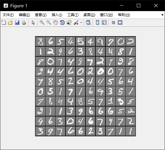
Part 1: Loading and Visualizing Data

• Load Training Data

1

load('ex3data1.mat'); % training data stored in arrays X, y

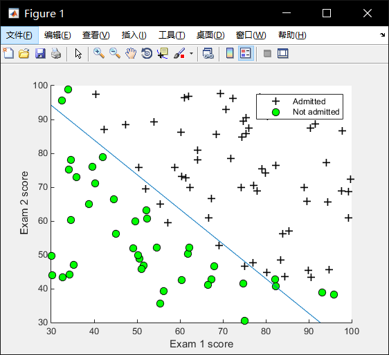
• Visualization

Part 2a: Vectorize Logistic Regression

• Compute the cost of a particular choice of theta. You should set J to the cost.
  Compute the partial derivatives and set grad to the partial derivatives of the cost w.r.t. each parameter in theta

1
2
3
4
5

J = (1 / m) * sum(-y .* log(sigmoid(X * theta)) - (1 - y) .* log(1 - sigmoid(X * theta))) + (lambda / (2 * m)) * sum(theta(2:size(theta)) .^2);

temp = theta;
temp(1) = 0;
grad = (1 / m) * (X' * (sigmoid(X * theta) - y)) + (lambda / m) * temp;

Part 2b: One-vs-All Training

• You should complete the following code to train num_labels logistic regression classifiers with regularization parameter lambda.

1
2
3
4
5
6

% Set Initial theta
initial_theta = zeros(n + 1, 1);
% Set options for fminunc
options = optimset('GradObj', 'on', 'MaxIter', 50);
for c = 1: num_labels
      all_theta(c, :) = fmincg (@(t)(lrCostFunction(t, X, (y == c), lambda)), initial_theta, options);

Part 3: Predict for One-Vs-All

• Complete the following code to make predictions using your learned logistic regression parameters (one-vs-all).

1
2

predict = sigmoid(X * all_theta');
[~,p] = max(predict, [], 2); % ~ means ignore this 1st parameter output

ex3_nn.m

• Complete the following code to make predictions using your learned neural network.

1
2
3
4
5
6

X = [ones(m, 1) X];
z1 = sigmoid(X * Theta1');
z1 = [ones(m, 1) z1];
z2 = sigmoid(z1 * Theta2');

[~, p] = max(z2, [], 2);

ex4.m

Part 3: Compute Cost (Feedforward)

• Feedforward the neural network and return the cost in the variable J. After implementing Part 1, you can verify that your cost function computation is correct by verifying the cost computed in ex4.m

1
2
3
4
5
6
7
8
9
10
11
12
13
14
15
16
17
18
19
20
21
22

% input layer
a1 = X;

% hidden layer
X = [ones(m, 1) X];  % 5000 * (1 + 400) = 5000 * 401
z2 = Theta1 * X'; % (25 * 401) * (401 * 5000) = 25 * 5000
a2 = sigmoid(z2); % 25 * 5000

% output layer
a2 = [ones(m, 1) a2']; % 5000 * (1 + 25) = 5000 * 26
z3 = Theta2 * a2'; % (10 * 26) * (26 * 5000) = 10 * 5000

% recode the labels as vectors containing only values 0 or 1
y_vec = zeros(num_labels, m); % 10 * 5000
% put value 1 for every iterated column
for i = 1: m
    y_vec(y(i), i) = 1;
end;

% cost function
h_theta = sigmoid(z3);
J = (-1 / m) * sum(sum(y_vec .* log(h_theta) + (1 - y_vec) .* log(1 - sigmoid(h_theta))));

Part 4: Implement Regularization

• You should now add regularization to your cost function. Notice that you can first compute the unregularized cost function J using your existing nnCostFunction.m and then later add the cost for the regularization terms.

1
2
3
4
5

% regularized cost function
theta1 = Theta1(:, 2:size(Theta1, 2)); % size(Theta1, 2) returns the nums of locumns in the matrix
theta2 = Theta2(:, 2:size(Theta2, 2));

J = J + lambda / (2 * m) * ( sum(sum(theta1 .^ 2)) + sum(sum(theta2 .^ 2)) ); % !sum up separately

Part 5: Sigmoid Gradient

• Implement the sigmoid gradient function

1

g = sigmoid(z) .* (1 - sigmoid(z));

Part 6: Initializing Pameters

• Initialize W randomly so that we break the symmetry while training the neural network

1
2
3

% Randomly initialize the weights to small values
epsilon_init = 0.12;
W = rand(L_out, 1 + L_in) * 2 * epsilon_init - epsilon_init;

Part 7: Implement Backpropagation

• Implement the backpropagation algorithm to compute the gradients Theta1_grad and Theta2_grad.

1
2
3
4
5
6
7
8
9
10
11
12
13
14
15
16
17
18
19
20
21
22
23
24
25
26

for t = 1:m
    % Step1
    a1 = X(t, :); % 1 * 401
    a1 = a1'; % 401 * 1
    z2 = Theta1 * a1; % (25 * 401) * (401 * 1) = 25 * 1
    a2 = sigmoid(z2); % 25 * 1
    
    a2 = [1; a2]; % add bais, (25 + 1) * 1 = 26 * 1
    z3 = Theta2 * a2; % (10 * 26) * (26 * 1) = 10 * 1
    a3 = sigmoid(z3); % 10 * 1
    
    % Step2
    delta_3 = a3 - y_vec(:, t); % 10 * 1

    % Step3
    delta_2 = (Theta2' * delta_3) .* sigmoidGradient([1; z2]); % add bais, 26 * 1
    
    % Step4
    delta_2 = delta_2(2: end); % 25 * 1
    
    Theta1_grad = Theta1_grad + delta_2 * a1'; % 10 * 25, !sum up grad
    Theta2_grad = Theta2_grad + delta_3 * a2'; % 10 * 25
end
    %Step5
    Theta1_grad = (1 / m) * Theta1_grad;
    Theta2_grad = (1 / m) * Theta2_grad;

Gradient checking

1
2
3
4
5
6
7
8
9
10
11
12
13

% take a look and try to understand
numgrad = zeros(size(theta));
perturb = zeros(size(theta));
e = 1e-4;
for p = 1:numel(theta)
    % Set perturbation vector
    perturb(p) = e;
    loss1 = J(theta - perturb);
    loss2 = J(theta + perturb);
    % Compute Numerical Gradient
    numgrad(p) = (loss2 - loss1) / (2*e);
    perturb(p) = 0;
end

Part 8: Implement Regularization

• Implement regularization with the cost function and gradients.

1
2

Theta1_grad(:, 2:end) = Theta1_grad(:, 2:end) + (lambda / m) * Theta1(:, 2:end);
Theta2_grad(:, 2:end) = Theta2_grad(:, 2:end) + (lambda / m) * Theta2(:, 2:end);

9. 回文数

• 给你一个整数 x ，如果 x 是一个回文整数，返回 true ；否则，返回 false 。
  • 回文数是指正序（从左向右）和倒序（从右向左）读都是一样的整数。例如，121 是回文，而 123 不是。

解题思路

借鉴第七题 7. 整数反转思想，取反后比较两数是否相同

代码

1
2
3
4
5
6
7
8
9
10
11
12

class Solution {
    public boolean isPalindrome(int x) {
        int temp = x;
        int sum = 0;
        while(temp > 0) {
            sum = sum * 10 + temp % 10;
            temp /= 10;
        }
        
        return sum == x ? true : false; 
    }
}

13. 罗马数字转整数

• 给定一个罗马数字，将其转换成整数。输入确保在 1 到 3999 的范围内。

  • I 可以放在 V (5) 和 X (10) 的左边，来表示 4 和 9。
  • X 可以放在 L (50) 和 C (100) 的左边，来表示 40 和 90。
  • C 可以放在 D (500) 和 M (1000) 的左边，来表示 400 和 900。

解题思路

• 一开始想法很复杂，考虑前后位置上的减法

• 后来借鉴思路是抓核心问题，对于第一个字符对应的数值，依次向后找，遇到比它还大的则减去，否则累加和。最后再处理最后一位上的加和，得到结果。

• 值得多斟酌，单个 for 循环，算法复杂度为 O (n)

代码

1
2
3
4
5
6
7
8
9
10
11
12
13
14
15
16
17
18
19
20
21
22
23
24
25
26
27
28

class Solution {
    public int romanToInt(String s) {
        int sum = 0;
        int num_former = transform(s.charAt(0));
        for (int i = 1; i < s.length(); i++) {
            int num_latter = transform(s.charAt(i));
            if(num_former < num_latter)
                sum -= num_former;
            else
                sum += num_former;
            num_former = num_latter;
        }
        return sum+num_former;
    }
    
    private int transform(char c) {
        switch(c){
            case 'I': return 1;
            case 'V': return 5;
            case 'X': return 10;
            case 'L': return 50;
            case 'C': return 100;
            case 'D': return 500;
            case 'M': return 1000;
            default: return 0;
        }
    }
}

ex1.m

Part 1: Basic Function

• Modify warmUpExercise.m to return a 5 x 5 identity matrix

1

A = eye(5);

Part 2: Plotting

• Plot the training data into a figure in plotData.m

1
2
3
4
5
6
7

data = load('ex1data1.txt')
x = data(:, 1);y = data(:,2)
m = length(y)

plot(x, y, 'rx', 'MarkerSize', 10);
ylabel('Profit in $10,000s')
xlabel('Population of City in 10,000s')

Part 3: Cost and Gradient descent

• complete the code in the file computeCost.m, which is a function that computes J(θ)

1

J = sum(((X * theta) - y).^2) / (2 * m);

• Perform a single gradient step on the parameter vector theta in gradientDescent.m

1
2

for iter = 1:num_iters
    theta = theta - alpha * (1 / m) * (X'* ((X * theta) - y) );

ex2.m

Part 1: Plotting

• Plot the positive and negative examples on a 2D plot, using the option ‘k+’ for the positive examples and ‘ko’ for the negative examples

1
2
3

positive = find(y == 1); negative = find(y == 0);
plot(X(positive, 1), X(positive, 2), 'k+','LineWidth', 1.2, 'MarkerSize', 8);
plot(X(negative, 1), X(negative, 2), 'ko','MarkerFaceColor', 'g', 'MarkerSize', 8);

Part 2: Compute Cost and Gradient

• Compute the sigmoid of each value of z (z can be a matrix, vector or scalar)

1
2

% Y = exp(X) 为数组 X 中的每个元素返回指数 e^x
g = 1 ./ (1 + exp(1) .^ (-z));

• Compute the cost of a particular choice of theta. You should set J to the cost

1
2
3

J = (1 / m) * sum(
	-y .* log(sigmoid(X * theta)) - (1 - y) .* log(1 - sigmoid(X * theta
)));

• Compute the partial derivatives and set grad to the partial derivatives of the cost w.r.t. each parameter in theta

1
2

for j = 1:size(theta)
    grad(j) = (1 / m) * sum((sigmoid(X * theta) - y) .* X(:, j));

Part 3: Optimizing using fminunc

Part 4: Predict and Accuracies

• Complete the following code to make predictions using your learned logistic regression parameters. You should set p to a vector of 0’s and 1’s

1

p = sigmoid(X * theta) >= 0.5;

ex2_reg.m

Part 1: Regularized Logistic Regression

• Compute the cost of a particular choice of theta. You should set J to the cost

  • tip: In Octave/MATLAB, recall that indexing starts from 1, hence, you should not be regularizing the theta(1) parameter (which corresponds to θ0) in the code

1

J = (1 / m) * sum(-y .* log(sigmoid(X * theta)) - (1 - y) .* log(1 - sigmoid(X * theta))) + (lambda / (2 * m)) * sum(theta(2:size(theta)) .^2);

• Compute the partial derivatives and set grad to the partial derivatives of the cost w.r.t. each parameter in theta

1
2
3

grad(1) = sum((sigmoid(X * theta) - y) .* X(:, 1)) / m;
for j = 2 : size(theta)
    grad(j) = sum((sigmoid(X * theta) - y) .* X(:, j)) / m + (lambda / m) * theta(j);

1. 两数之和

• 给定一个整数数组 nums 和一个整数目标值 target，请你在该数组中找出 和为目标值 target 的那 两个 整数，并返回它们的数组下标。
  • 你可以假设每种输入只会对应一个答案。但是，数组中同一个元素在答案里不能重复出现。
  • 你可以按任意顺序返回答案。

解题思路

1. 嵌套循环暴力求解，算法复杂度为 O (n^2)
2. 使用 Hashmap，算法复杂度为 O (n)

代码

• 解法一

1
2
3
4
5
6
7
8
9
10
11
12
13
14
15
16
17
18

class Solution {
    public int[] twoSum(int[] nums, int target) {
        int num1 = 0;
        int num2 = 0;
        int[] result = new int[2];
        for(int i = 0; i < nums.length; i++){
            num1 = nums[i];
            for(int j = i+1; j < nums.length; j++){
                num2 = nums[j];
                if(num1+ num2 == target){
                    result[0] = i;
                    result[1] = j;
                }     
            }
        }
        return result;
    }
}

• 解法二

1
2
3
4
5
6
7
8
9
10
11
12
13
14
15

class Solution {
    public int[] twoSum(int[] nums, int target) {
        int[] res = new int[2];
        Map<Integer, Integer> map = new HashMap<>();
        for (int i = 0; i < nums.length; i++) {
            int temp = target - nums[i];
            if(map.containsKey(temp)){
                res[0] = map.get(temp);
                res[1] = i;
            } else
                map.put(nums[i], i);
        }
        return res;
    }
}

7. 整数反转

• 给你一个 32 位的有符号整数 x ，返回将 x 中的数字部分反转后的结果。

  • 如果反转后整数超过 32 位的有符号整数的范围 [−231, 231 − 1] ，就返回 0。
  • 假设环境不允许存储 64 位整数（有符号或无符号）。

解题思路

主要难点在于数据类型范围，考虑先处理正负，再在同个循环内部同时完成取当前位值和累加反转值操作，最后处理结果

代码

1
2
3
4
5
6
7
8
9
10
11
12
13
14
15
16
17
18
19

class Solution {
    public int reverse(int x) {
        boolean flag = false;
        if(x < 0){
            flag = true;
            x = -x;
        }

        int sum = 0;
        while(x > 0) {
            if (sum > (Integer.MAX_VALUE - x % 10) / 10)
                return 0;
            sum = sum * 10 + x % 10;
            x /= 10;
        }
    
        return flag ? -sum : sum;
    }
}

第七章 复用类

1、复用的方法

• 在新类中产生现有类的对象

• 继承

2、组合语法

• 将对象引用置于新类

• 初始化引用的位置

  • 定义处
  • 类构造器中
  • 惰性初始化（Delay Initialization）于使用对象前

3、继承

• 声明新类与旧类类似

  • 书写紧跟基类名称关键字 extends

• super 为超类，类从超类继承

• 使用 += 可连接多个 String 对象

• 构建过程（初始化过程同）是向外 “扩散” 的

  • 若类带有参数，则需要用 super 显式编写调用

4、代理：继承与组合的中间体

• 异同：组合将成员对象置于要构造类中，但在新类中暴露了成员对象的所有方法；相较之，代理使用接口，这样与继承得到的接口相同而又只提供成员对象的某个子集，从而得到更多的控制力

• java 不直接支持代理，可使用部分支持 ide 自动生成

5、结合使用组合和继承

• finally () 子句确保正确清理，采用自己编写的顺序清理

• dispose ()：清理方法

• 无名称屏蔽：重载方法不会屏蔽基类方法（区别 C++）

  • 需要覆写：Override ()，不是关键字但按关键字处理

对比

• 组合显式允许在新类中放置子类，但继承为隐式创建

• 组合适用于在新类中使用现有类的功能而非接口，继承反之

• 组合允许直接访问新类中的组合成分（public），继承相对更为安全且易于理解端口

• is-a 关系 - 继承，has-a 关系 - 组合

6、protected 关键字

• 提供包内和继承于此类的导出类的访问权限，对类用户私密

7、final 关键字

• 对数据使用：编译时常量 或 运行时被初始化的值

• 类常量 static final